Remote Sensing of the Environment: Miscellaneous Image Functions

Remote Sensing Lab 4

Goals and Background

Lab 4 guides students thru a series of Miscellaneous Image Functions using Eradis Imagine 2016 to gain skills in:

• Image processing
• Enhancing images for visual interpretation
• Delinage any study are (area of interest) from a larger satellite image
• Mosiac multiple image scenes
• Construct a simple graphical model for remote sensing analytics

Methods

Part 1: Image Subsetting

Clipping an remotely sensed image to a smaller area of interest (AOI) is important for image processing. Processing time increases with pixel volume, so by cutting to a smaller AOI you cut processing time. To achieve this, I used two methods:

• Creation of rectangular box using the Inquire Box
• Delineate an Area of Interest
• Allows subsetting images that are not rectangular, like the shape of a county for example.

Part 2: Image Fusion

Images are fused together for a number of different reasons. In this excercize I conducted a Pan Sharpen Resolution Merge. I began with two images; a high resolution panchromatic (grey scale) image and a lower resolution multispectral (RGB, color) image of the same location. The image fusion combines the two images so that the resolution of the panchromatic image is maintained, but color is added to it. Nearest neighbor resampling was utlized.  

Part 3: Simple Radiometric Enhancement Techniques

Several radiometric enhancement techniques are used improve the spectral or radiometric quality of a raster image. For this lab we experimented with the Haze Reduction tool to remove clouds in an image.

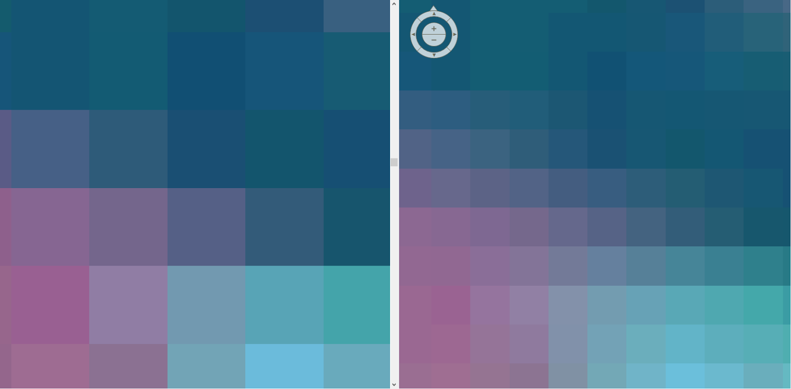
Part 4: Linking Image Viewer to Google Earth

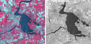
While Erdas Imagine, the analyzer can use the 'Connect to Google Earth' tool which pulls up a Google Earth browser. This browser can be displayed side-by-side with a raster image to be analyzed, linked, and synced with it so that the two viewers move over the same geography simultaneously. 

Part 5: Resampling

Resampling is altering the size of pixels of an image to increase pixel size (resample down) or reduce pixel size (resample up) depending on analytical demands. To practice this skill using an aerial photograph of Eau Claire, I resampled up, or reduced the pixel size from 30m to 15m. This was achieved using two different methods:

• Nearest Neighbor
• Bilinear Interpolation

Part 6: Image Mosaicking

Mosaicking is a necessary function for when an area of interest is larger than the available raster, or straddles the edges of two raster swats. The process blends the two images together so that they can be analyzed seamlessly. While there are multiple methods for doing this, we experimented with two of them:

• Mosaic Express - select the upper and lower image and the function does the rest.
• Mosaic Pro - this option takes longer, but provides a variety of options and flexibility so that the result of the mosaic can be as seamless as possible.

Part 7: Binary Change Detection

It is often valuable to analyze raster images of the same location taken from different points in time to analyze change over time. For this we estimated and mapped the brightness values of pixels that changed in Eau Claire and four neighboring counties between August 1991 and August 2011. This process required many steps.

1. Create a Difference Image: Use functions > Two Input Operators tool to subtract the two rasters.
2. Map Change Pixels in Output
1. Use Spatial Modeler to compute this equation: Change in Pixel Values = Brightness values of 2011 image - Brightness values of 1991 image + constant (to avoid negative numbers)
2. Analyze the histogram of this output to find the change/no change threshold
3. Use Spatial Modeler to compute this equation: Either 1 IF (<input>change/no change threshold value) OR 0 OTHERWISE. This shows all pixels above the threshold and masks those below it.
3. Use resulting raster to create a map in ArcMap displaying the change and no change areas in this section of Wisconsin over the last 20 years.  

Results

Part 1: Subsetting Outputs

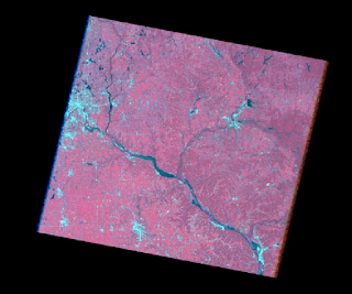Figure 1: Initial image eau_claire_2011

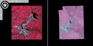Figure 2: Image Outputs. Left, using Inquire Box Method to subset the cities of Eau Claire and Chippewa. Right, using Area of Interest Delineation to subset Eau Claire and Chippewa Counties. 

Part 2: Fusion Outputs

Figure 3 Image Inputs. Left, multispectral image with 30m resolution. Right, panchromatic image with 15m resolution.

Figure 4 Image Output. Left, original multispectral image with 30m resolution. Right, pansharpened fusion image with 15m resolution.

Part 3: Radiometric Enhancement Outputs

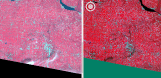Figure 5: Left: Image input. Notice the white haze/cloud and black shadow.
Right: Image output. Notice that the white haze/cloud has disappeared, but the black shadow remains. Further image processing would be required to remedy this. 

Part 4: Linking Image Viewer

There were no outputs for this portion of the lab, however it was determined that Google Earth makes an excellent selective key when linked to the image viewer. 

Part 5: Resampling Outputs

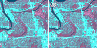Figure 6: Resampling with Nearest Neighbor. Original image on left, output on right. There are few changes in appearance; pixels are shifted up slightly.

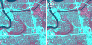Figure 7: Resampling with Bilinear Interpolation. Original image on left, output on right. Notice that the objects in the resampled image have smoother (less jagged) edges. 

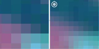Figure 8: Zoomed in Resampling with Bilinear Interpolation. Original image on left, output on right. Notice that the resampled image has pixels that are approximately 1/4 the size of the pixels in the original image, which makes sense given that 15m^2 is 1/4 the size of  30m^2.

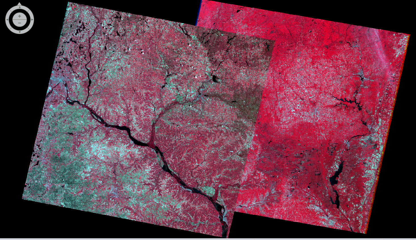
Part 6: Image Mosaicking

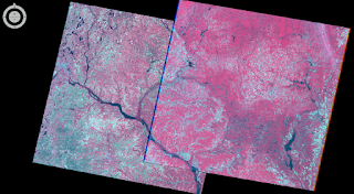Figure 9: Original images to be mosaicked.

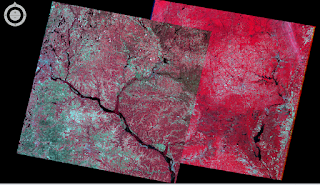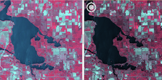
Figure 10: Mosiac output using Mosiac Express. Notice sharp contrast line between the two images.

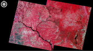Figure 11: Mosiac output using Mosiac Pro. With histogram matching and overly, there is much smoother transition from one image to the next. 

Part 7: Binary Change Detection

Two Input Operators Method:

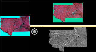Figure 12: Left, Eau Claire 1991. Top right, Eau Claire 2011. Bottom right, output image.

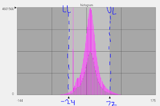Figure 13: Output Image Histogram. Lower Limit: -24, Upper Limit: 72

Spatial Modeler Method:

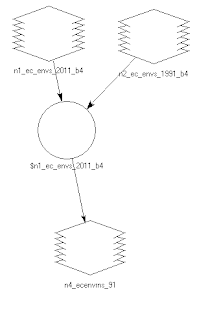Figure 14: Model 1, used to find the difference between two input rasters. The two input rasters are Eau Claire 1991 and Eau Claire 2011, as depicted in Figure 12

Figure 14: Output of Model 1. Analyzed Histogram for mean and standard deviation to find the change/no change threshold value (202.186).

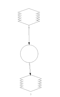Figure 15: Model 2, used to generate a raster showing all pixels above the 202.186 and mask out those below the 202.186. Input raster is the Output of Model 1, depicted in Figure 14. Function: EITHER 1 IF ($n1_ec_91 > 202.186) OR 0 OTHERWISE. Ouput depicted in Figure 16.

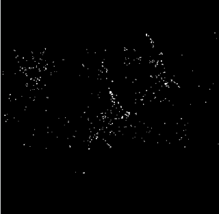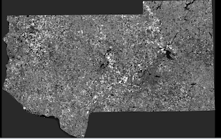
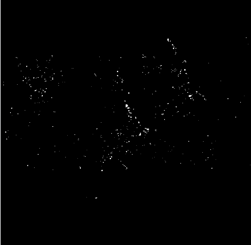
Figure 16: Output of Model 2. White spots represents areas of change.

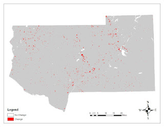Image 16: Map representation of Output of Model 2, where red represents change and grey represents no change. 

Sources

No sources outside of those provided by instructor were used. These sources included Lab Directions and input images.