Remote Sensing Lab 5
Goals and Background
The goal of this lab was to practice using LiDAR data and become familiar with associated geoprocessing techniques in ArcMap. This includes the processing and retrieval of various surface and terrain models, and the processing and creation of an intensity image and other derivative products from the point cloud.
LiDAR, which stands for Light Detection and Ranging, is a rapidly expanding area of remote sensing where distance to a target is detected with a laser light. Between 200 to 400,000 pulses are emitted per second, and their echos are collected a receiving system that calculates precise X, Y, and Z coordinates for objects and surfaces on earth.
To explore LiDAR data and common geoprocessing techniques, I used LiDAR data collected by Ayres Associates in 2013 for the county of Eau Claire. The data covers 567 square miles and was collected with a Riegl sensor mounted to a fixed-wing aircraft. Specific location of data collected using PLSS: (13-27-10SE, 24-27-10NE, 24-27-10SE, 25-27-10NE, 25-27-10SE,
15-27-09SW, 22-27-09NW, 22-27-09SW, 27-27-09NW, 27-27-09SW, 16-27-09SE, 16-27-09SW,
17-27-09SE, 17-27-09SW, 18-27-09SE, 18-27-09SW, 21-27-09NE, 21-27-09SE, 21-27-09NW,
21-27-09SW, 20-27-09NE, 20-27-09NE, 20-27-09NW, 20-27-09SW, 19-27-09NE, 19-27-09SE,
19-27-09NW, 19-27-09SW, 28-27-09NE, 28-27-09SE, 28-27-09NW, 28-27-09SW, 29-27-09NE,
29-27-09SE, 29-27-09NW, 29-27-09SW, 30-27-09NE, 30-27-09SE, 30-27-09NW, 30-27-09SW)
Methods
Create New LAS Dataset
In ArcMap catalog, I created a new LAS Dataset named Eau_Claire_City.lasd. The dataset is populated with the files provided by Ayres Associates. Using metadata provided by Ayres Associates I determined the horizontal and vertical coordinate system and defined those of the new dataset to match.
Use LAS Dataset Toolbar to experiment with Data Symbology
After turning on 3D Analysy and Spatial Analyst, I was able to use the LAS Dataset Toolbar to experiment with the symbology of Eau_Claire_City.lasd. Data can be configured to show aspect, slope, and contours of the area (Figure 1).
Using the LAS Dataset Profile View tool allows the user to draw a box around a particular area and view that object in a crossectional view rather than in map view (Figure 2).
Using the LAS Dataset Profile View tool allows the user to draw a box around a particular area and view that object in a crossectional view rather than in map view (Figure 2).
Generation of LiDAR Derivative Products
Using the LAS Dataset to Raster tool, I created a Digital Surface model (DSM) using first return (Figure 3), Digital terrain model (DTM) (Figure 4), and a hillshade of the DSM (Figure 5) and DTM (Figure 6).
Also using the LiDAR to Raster too, I created a LiDAR intensity image using Points and the Filter set as First Return (Figure 7). The image appears dark, so I also opened it in Erdas Imagine which automatically enhanced its display (Figure 8).
Results


 |
| Figure 1. Centering above UW Eau Claire and the third ward, Eau_Claire_City.lasd symbolized to show Aspect (top), Slope (middle), and Contour (bottom). |
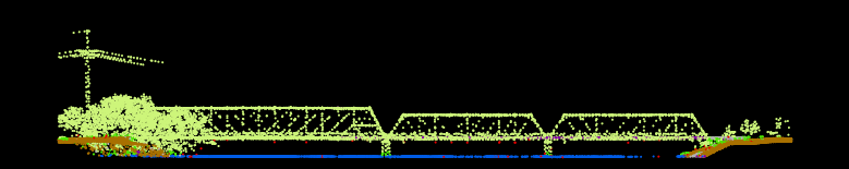 |
| Figure 2. Map View of the Phoenix Park bridge crossing the Chippewa River. |
 |
| Figure 3. Eau Claire Digital Surface Model |
 |
| Figure 4. Eau Claire Digital Terrain Model |
 |
| Figure 5. Hillshade of Digital Surface Model |
 |
| Figure 6. Hillshade of Digital Terrain Model |
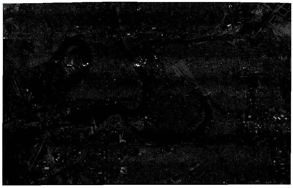 |
| Figure 7. LiDar Intensity Image in ArcMap |
 |
| Figure 8. Enhanced LiDar Intensity Image in Erdas Imagine. |
No comments:
Post a Comment